About this article: it originated as a series of posts on the Communications of the ACM blog. I normally repost such articles here. (Even though copy-paste is usually not good, there are three reasons for this duplication: the readership seems to be largely disjoint; I can use better formatting, since their blog software is more restrictive than WordPress; and it is good to have a single repository for all my articles, including both those who originated on CACM and those who did not.) The series took the form of nine articles, where each of the first few ended with a quiz, to which the next one, published a couple of days later, provided an answer. Since all these answers are now available it would make no sense to use the same scheme, so I am instead publishing the whole thing as a single article with nine sections, slightly adapted from the original.
I was too lazy so far to collect all the references into a single list, so numbers such as [1] refer to the list at the end of the corresponding section.
A colleague recently asked me to present a short overview of axiomatic semantics as a guest lecture in one of his courses. I have been teaching courses on software verification for a long time (see e.g. here), so I have plenty of material; but instead of just reusing it, I decided to spend a bit of time on explaining why it is good to have a systematic approach to software verification. Here is the resulting tutorial.
1. Introduction and attempt #1
Say “software verification” to software professionals, or computer science students outside of a few elite departments, and most of them will think “testing”. In a job interview, for example, show a loop-based algorithm to a programmer and ask “how would you verify it?”: most will start talking about devising clever test cases.
Far from me to berate testing [1]; in fact, I have always thought that the inevitable Dijkstra quote about testing — that it can only show the presence of errors, not their absence [2] — which everyone seems to take as an indictment and dismissal of testing (and which its author probably intended that way) is actually a fantastic advertisement for testing: a way to find bugs? Yes! Great! Where do I get it? But that is not the same as verifying the software, which means attempting to ascertain that it has no bugs.
Until listeners realize that verification cannot just mean testing, the best course material on axiomatic semantics or other proof techniques will not attract any interest. In fact, there is somewhere a video of a talk by the great testing and public-speaking guru James Whittaker where he starts by telling his audience not to worry, this won’t be a standard boring lecture, he will not start talking about loop invariants [3]! (Loop invariants are coming in this article, in fact they are one of its central concepts, but in later sections only, so don’t bring the sleeping bags yet.) I decided to start my lecture by giving an example of what happens when you do not use proper verification. More than one example, in fact, as you will see.
A warning about this article: there is nothing new here. I am using an example from my 1990 book Introduction to the Theory of Programming Languages (exercise 9.12). Going even further back, a 1983 “Programming Pearls” Communications of the ACM article by Jon Bentley [4] addresses the same example with the same basic ideas. Yet almost forty years later these ideas are still not widely known among practitioners. So consider these articles as yet another tutorial on fundamental software engineering stuff.
The tutorial is a quiz. We start with a program text:
from
i := 1 ; j := n — Result initialized to 0.
until i = j loop
m := (i + j) // 2 — Integer division
if t [m] ≤ x then i := m else j := m end
end
if x = t [i] then Result := i end
All variables are of integer type. t is an up-sorted array of integers, indexed from 1 to n . We do not let any notation get between friends. A loop from p until e loop q end executes p then, repeatedly: stops if e (the exit condition) is true, otherwise executes q. (Like {p ; while not e do {q}} in some other notations.) “:=” is assignment, “=” equality testing. “//” is integer division, e.g. 6 //3 = 7 //3 = 2. Result is the name of a special variable whose final value will be returned by this computation (as part of a function, but we only look at the body). Result is automatically initialized to zero like all integer variables, so if execution does not assign anything to Result the function will return zero.
First question: what is this program trying to do?
OK, this is not the real quiz. I assume you know the answer: it is an attempt at “binary search”, which finds an element in the array, or determines its absence, in a sequence of about log2 (n) steps, rather than n if we were use sequential search. (Remember we assume the array is sorted.) Result should give us a position where x appears in the array, if it does, and otherwise be zero.
Now for the real quiz: does this program meet this goal?
The answer should be either yes or no. (If no, I am not asking for a correct version, at least not yet, and in any case you can find some in the literature.) The situation is very non-symmetric, we might say Popperian:
- To justify a no answer it suffices of a single example, a particular array t and a particular value x, for which the program fails to set Result as it should.
- To justify a yes answer we need to provide a credible argument that for every t and x the program sets Result as it should.
Notes to section 1
[1] The TAP conference series (Tests And Proofs), which Yuri Gurevich and I started, explores the complementarity between the two approaches.
[2] Dijkstra first published his observation in 1969. He did not need consider the case of infinite input sets: even for a trivial finite program that multiplies two 32-bit integers, the number of cases to be examined, 264, is beyond human reach. More so today with 64-bit integers. Looking at this from a 2020 perspective, we may note that exhaustive testing of a finite set of cases, which Dijkstra dismissed as impossible in practice, is in fact exactly what the respected model checking verification technique does; not on the original program, but on a simplified — abstracted — version precisely designed to keep the number of cases tractable. Dijkstra’s argument remains valid, of course, for the original program if non-trivial. And model-checking does not get us out of the woods: while we are safe if its “testing” finds no bug, if it does find one we have to ensure that the bug is a property of the original program rather than an artifact of the abstraction process.
[3] It is somewhere on YouTube, although I cannot find it right now.
[4] Jon Bentley: Programming Pearls: Writing Correct Programs, in Communications of the ACM, vol. 26, no. 12, pp. 1040-1045, December 1983, available for example here.
2. Attempt #2
Was program #1 correct? If so it should yield the correct answer. (An answer is correct if either Result is the index in t of an element equal to x, or Result = 0 and x does not appear in t.)
This program is not correct. To prove that it is not correct it suffices of a single example (test case) for which the program does not “yield the correct answer”. Assume x = 1 and the array t has two elements both equal to zero (n = 2, remember that arrays are indexed from 1):
t = [0 0]
The successive values of the variables and expressions are:
m i j i + j + 1
After initialization: 1 2 3
i ≠ j, so enter loop: 1 1 2 6 — First branch of “if” since t [1] ≤ x
— so i gets assigned the value of m
But then neither of the values of i and j has changed, so the loop will repeat its body identically (taking the first branch) forever. It is not even that the program yields an incorrect answer: it does not yield an answer at all!
Note (in reference to the famous Dijkstra quote mentioned in the first article), that while it is common to pit tests against proofs, a test can actually be a proof: a test that fails is a proof that the program is incorrect. As valid as the most complex mathematical proof. It may not be the kind of proof we like most (our customers tend to prefer a guarantee that the program is correct), but it is a proof all right.
We are now ready for the second attempt:
— Program attempt #2.
from
i := 1 ; j := n
until i = j or Result > 0 loop
m := (i + j) // 2 — Integer division
if t [m] ≤ x then
i := m + 1
elseif t [m] = x then
Result := m
else — In this case t [m] > x
j := m – 1
end
end
Unlike the previous one this version always changes i or j, so we may hope it does not loop forever. It has a nice symmetry between i and j.
Same question as before: does this program meet its goal?
3. Attempt #3
The question about program #2, as about program #1: was: it right?
Again no. A trivial example disproves it: n = 1, the array t contains a single element t [1] = 0, x = 0. Then the initialization sets both i and j to 1, i = j holds on entry to the loop which stops immediately, but Result is zero whereas it should be 1 (the place where x appears).
Here now is attempt #3, let us see it if fares better:
— Program attempt #3.
from
i := 1 ; j := n
until i = j loop
m := (i + j + 1) // 2
if t [m] ≤ x then
i := m + 1
else
j := m
end
end
if 1 ≤ i and i ≤ n then Result := i end
— If not, Result remains 0.
What about this one?
3. Attempt #4 (also includes 3′)
The first two program attempts were wrong. What about the third?
I know, you have every right to be upset at me, but the answer is no once more.
Consider a two-element array t = [0 0] (so n = 2, remember that our arrays are indexed from 1 by convention) and a search value x = 1. The successive values of the variables and expressions are:
m i j i + j + 1
After initialization: 1 2 4
i ≠ j, so enter loop: 2 3 2 6 — First branch of “if” since t [2] < x
i ≠ j, enter loop again: 3 ⚠ — Out-of-bounds memory access!
— (trying to access non-existent t [3])
Oops!
Note that we could hope to get rid of the array overflow by initializing i to 0 rather than 1. This variant (version #3′) is left as a bonus question to the patient reader. (Hint: it is also not correct. Find a counter-example.)
OK, this has to end at some point. What about the following version (#4): is it right?
— Program attempt #4.
from
i := 0 ; j := n + 1
until i = j loop
m := (i + j) // 2
if t [m] ≤ x then
i := m + 1
else
j := m
end
end
if 1 ≤ i and i ≤ n then Result := i end
5. Attempt #5
Yes, I know, this is dragging on. But that’s part of the idea: witnessing how hard it is to get a program right if you just judging by the seat of your pants. Maybe we can get it right this time?
Are we there yet? Is program attempt #4 finally correct?
Sorry to disappoint, but no. Consider a two-element array t = [0 0], so n = 2, and a search value x = 1 (yes, same counter-example as last time, although here we could also use x = 0). The successive values of the variables and expressions are:
m i j i + j
After initialization: 0 3 3
i ≠ j, so enter loop: 1 2 3 5 — First branch of “if”
i ≠ j, enter loop again: 2 3 3 6 — First branch again
i = j, exit loop
The condition of the final “if” is true, so Result gets the value 3. This is quite wrong, since there is no element at position 3, and in any case x does not appear in t.
But we are so close! Something like this should work, should it not?
So patience, patience, let us tweak it just one trifle more, OK?
— Program attempt #5.
from
i := 1 ; j := n + 1
until i ≥ j or Result > 0 loop
m := (i + j) // 2
if t [m] < x then
i := m + 1
elseif t [m] > x then
j := m
else
Result := m
end
end
Does it work now?
6. Attempt #6
The question about program #5 was the same as before: is it right, is it wrong?
Well, I know you are growing more upset at me with each section, but the answer is still that this program is wrong. But the way it is wrong is somewhat specific; and it applies, in fact, to all previous variants as well.
This particular wrongness (fancy word for “bug”) has a history. As I pointed out in the first article, there is a long tradition of using binary search to illustrate software correctness issues. A number of versions were published and proved correct, including one in the justly admired Programming Pearls series by Jon Bentley. Then in 2006 Joshua Bloch, then at Google, published a now legendary blog article [2] which showed that all these versions suffered from a major flaw: to obtain m, the approximate mid-point between i and j, they compute
(i + j) // 2
which, working on computer integers rather than mathematical integers, might overflow! This in a situation in which both i and j, and hence m as well, are well within the range of the computer’s representable integers, 2-n to 2n (give or take 1) where n is typically 31 or, these days, 63, so that there is no conceptual justification for the overflow.
In the specification that I have used for this article, i starts at 1, so the problem will only arise for an array that occupies half of the memory or more, which is a rather extreme case (but still should be handled properly). In the general case, it is often useful to use arrays with arbitrary bounds (as in Eiffel), so we can have even a small array, with high indices, for which the computation will produce an overflow and bad results.
The Bloch gotcha is a stark reminder that in considering the correctness of programs we must include all relevant aspects and consider programs as they are executed on a real computer, not as we wish they were executed in an ideal model world.
(Note that Jon Bentley alluded to this requirement in his original article: while he did not explicitly mention integer overflow, he felt it necessary to complement his proof by the comment that that “As laborious as our proof of binary search was, it is still unfinished by some standards. How would you prove that the program is free of runtime errors (such as division by zero, word overflow, or array indices out of bounds)?” Prescient words!)
It is easy to correct the potential arithmetic overflow bug: instead of (i + j) // 2, Bloch suggested we compute the average as
i + (j – i) // 2
which is the same from a mathematician’s viewpoint, and indeed will compute the same value if both variants compute one, but will not overflow if both i and j are within range.
So we are ready for version 6, which is the same as version 5 save for that single change:
— Program attempt #6.
from
i := 1 ; j := n + 1
until i ≥ j or Result > 0 loop
m := i + (j – i) // 2
if t [m] < x then
i := m + 1
elseif t [m] > x then
j := m
else
Result := m
end
end
Now is probably the right time to recall the words by which Donald Knuth introduces binary search in the original 1973 tome on Sorting and Searching of his seminal book series The Art of Computer Programming:
Although the basic idea of binary search is comparatively straightforward, the details can be somewhat tricky, and many good programmers have done it wrong the first few times they tried.
Do you need more convincing? Be careful what you answer, I have more variants up my sleeve and can come up with many more almost-right-but-actually-wrong program attempts if you nudge me. But OK, even the best things have an end. This is not the last section yet, but that was the last program attempt. To the naturally following next question in this running quiz, “is version 6 right or wrong”, I can provide the answer: it is, to the best of my knowledge, a correct program. Yes! [3].
But the quiz continues. Since answers to the previous questions were all that the programs were not correct, it sufficed in each case to find one case for which the program did not behave as expected. Our next question is of a different nature: can you find an argument why version #6 is correct?
References for section 6
[1] (In particular) Jon Bentley: Programming Pearls — Writing Correct Programs, in Communications of the ACM, vol. 26, no. 12, December 1983, pages 1040-1045, available here.
[2] Joshua Bloch: Extra, Extra — Read All About It: Nearly All Binary Searches and Mergesorts are Broken, blog post, on the Google AI Blog, 2 June 2006, available here.
[3] A caveat: the program is correct barring any typos or copy-paste errors — I am starting from rigorously verified programs (see the next posts), but the blogging system’s UI and text processing facilities are not the best possible for entering precise technical text such as code. However carefully I check, I cannot rule out a clerical mistake, which of course would be corrected as soon as it is identified.
7. Using a program prover
Preceding sections presented candidate binary search algorithms and asked whether they are correct. “Correct” means something quite precise: that for an array t and a value x, the final value of the variable Result is a valid index of t (that is to say, is between 1 and n, the size of t) if and only if x appears at that index in t.
The last section boldly stated that program attempt #6 was correct. The question was: why?
In the case of the preceding versions, which were incorrect, you could prove that property, and I do mean prove, simply by exhibiting a single counter-example: a single t and x for which the program does not correctly set Result. Now that I asserting the program to be correct, one example, or a million examples, do not suffice. In fact they are almost irrelevant. Test as much as you like and get correct results every time, you cannot get rid of the gnawing fear that if you had just tested one more time after the millionth test you would have produced a failure. Since the set of possible tests is infinite there is no solution in sight [1].
We need a proof.
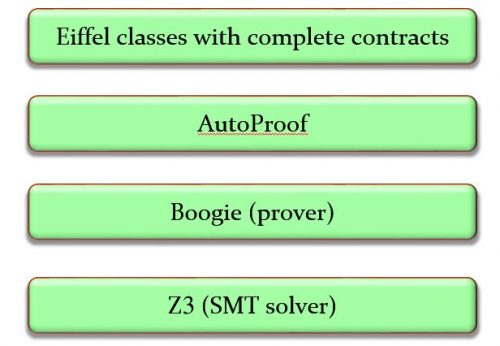
I am going to explain that proof in the next section, but before that I would like to give you an opportunity to look at the proof by yourself. I wrote in one of the earlier articles that most of what I have to say was already present in Jon Bentley’s 1983 Programming Pearls contribution [2], but a dramatic change did occur in the four decades since: the appearance of automated proof system that can handle significant, realistic programs. One such system, AutoProof, was developed at the Chair of Software engineering at ETH Zurich [3] (key project members were Carlo Furia, Martin Nordio, Nadia Polikarpova and Julian Tschannen, with initial contributions by Bernd Schoeller) on the basis of the Boogie proof technology from Microsoft Research).
AutoProof is available for online use, and it turns out that one of the basic tutorial examples is binary search. You can go to the corresponding page and run the proof.
I am going to let you try this out (and, if you are curious, other online AutoProof examples as well) without too many explanations; those will come in the next section. Let me simply name the basic proof technique: loop invariant. A loop invariant is a property INV associated with a loop, such that:
- A. After the loop’s initialization, INV will hold.
- B. One execution of the loop’s body, if started with INV satisfied (and the loop’s exit condition not satisfied, otherwise we wouldn’t be executing the body!), satisfies INV again when it terminates.
This idea is of course the same as that of a proof by induction in mathematics: the initialization corresponds to the base step (proving that P (0) holds) and the body property to the induction step (proving that from P (n) follows P (n + 1). With a traditional induction proof we deduce that the property (P (n)) holds for all integers. For the loop, we deduce that when the loop finishes its execution:
- The invariant still holds, since executing the loop means executing the initialization once then the loop body zero or more times.
- And of course the exit condition also holds, since otherwise we would still be looping.
That is how we prove the correctness of a loop: the conjunction of the invariant and the exit condition must yield the property that we seek (in the example, the property, stated above of Result relative to t and x).
We also need to prove that the loop does terminate. This part involves another concept, the loop’s variant, which I will explain in the next section.
For the moment I will not say anything more and let you look at the AutoProof example page (again, you will find it here), run the verification, and read the invariant and other formal elements in the code.
To “run the verification” just click the Verify button on the page. Let me emphasize (and emphasize again and again and again) that clicking Verify will not run the code. There is no execution engine in AutoProof, and the verification does not use any test cases. It processes the text of the program as it appears on the page and below. It applies mathematical techniques to perform the proof; the core property to be proved is that the proposed loop invariant is indeed invariant (i.e. satisfies properties A and B above).
The program being proved on the AutoProof example page is version #6 from the last section, with different variable names. So far for brevity I have used short names such as i, j and m but the program on the AutoProof site applies good naming practices with variables called low, up, middle and the like. So here is that version again with the new variable names:
— Program attempt #7 (identical to #6 with different variable names) .
from
low := 0 ; up := n
until low ≥ up or Result > 0 loop
middle := low + ((up – low) // 2)
if a [middle] < value then — The array is now called a rather than t
low := middle + 1
elseif a [middle] > value then
up := middle
else
Result := middle
end
end
This is exactly the algorithm text on the AutoProof page, the one that you are invited to let AutoProof verify for you. I wrote “algorithm text” rather than “program text” because the actual program text (in Eiffel) includes variant and invariant clauses which do not affect the program’s execution but make the proof possible.
Whether or not these concepts (invariant, variant, program proof) are completely new to you, do try the prover and take a look at the proof-supporting clauses. In the next article I will remove any remaining mystery.
Note and references for section 7
[1] Technically the set of possible [array, value] pairs is finite, but of a size defying human abilities. As I pointed out in the first section, the “model checking” and “abstract interpretation” verification techniques actually attempt to perform an exhaustive test anyway, after drastically reducing the size of the search space. That will be for some other article.
[2] Jon Bentley: Programming Pearls: Writing Correct Programs, in Communications of the ACM, vol. 26, no. 12, pp. 1040-1045, December 1983, available for example here.
[3] The AutoProof page contains documentations and numerous article references.
8. Understanding the proof
The previous section invited you to run the verification on the AutoProof tutorial page dedicated to the example. AutoProof is an automated proof system for programs. This is just a matter of clicking “Verify”, but more importantly, you should read the annotations added to the program text, particularly the loop invariant, which make the verification possible. (To avoid any confusion let me emphasize once more that clicking “Verify” does not run the program, and that no test cases are used; the effect is to run the verifier, which attempts to prove the correctness of the program by working solely on the program text.)
Here is the program text again, reverting for brevity to the shorter identifiers (the version on the AutoProof page has more expressive ones):
from
i := 1 ; j := n + 1
until i ≥ j or Result > 0 loop
m := i + (j – i) // 2
if t [m] < x then
i := m + 1
elseif t [m] > x then
j := m
else
Result := m
end
end
Let us now see what makes the proof possible. The key property is the loop invariant, which reads
A: 1 ≤ i ≤ j ≤ n + 1
B: 0 ≤ Result ≤ n
C: ∀ k: 1 .. i –1 | t [k] < x
D: ∀ k: j .. n | t [k] > x
E: (Result > 0) ⇒ (t [Result] = x)
The notation is slightly different on the Web page to adapt to the Eiffel language as it existed at the time it was produced; in today’s Eiffel you can write the invariant almost as shown above. Long live Unicode, allowing us to use symbols such as ∀ (obtained not by typing them but by using smart completion, e.g. you start typing “forall” and you can select the ∀ symbol that pops up), ⇒ for “implies” and many others
Remember that the invariant has to be established by the loop’s initialization and preserved by every iteration. The role of each of its clauses is as follows:
- A: keep the indices in range.
- B: keep the variable Result, whose final value will be returned by the function, in range.
- C and D: eliminate index intervals in which we have determined that the sought value, x, does not appear. Before i, array values are smaller; starting at j, they are greater. So these two intervals, 1..i and j..n, cannot contain the sought value. The overall idea of the algorithm (and most other search algorithms) is to extend one of these two intervals, so as to narrow down the remaining part of 1..n where x may appear.
- E: express that as soon as we find a positive (non-zero) Result, its value is an index in the array (see B) where x does appear.
Why is this invariant useful? The answer is that on exit it gives us what we want from the algorithm. The exit condition, recalled above, is
i ≥ j or Result > 0
Combined with the invariant, it tells us that on exit one of the following will hold:
- Result > 0, but then because of E we know that x appears at position Result.
- i < j, but then A, C and D imply that x does not appear anywhere in t. In that case it cannot be true that Result > 0, but then because of B Result must be zero.
What AutoProof proves, mechanically, is that under the function’s precondition (that the array is sorted):
- The initialization ensures the invariant.
- The loop body, assuming that the invariant is satisfied but the exit condition is not, ensures the loop invariant again after it executes.
- The combination of the invariant and the exit condition ensures, as just explained, the postcondition of the function (the property that Result will either be positive and the index of an element equal to x, or zero with the guarantee that x appears nowhere in t).
Such a proof guarantees the correctness of the program if it terminates. We (and AutoProof) must prove separately that it does terminate. The technique is simple: find a “loop variant”, an integer quantity v which remains non-negative throughout the loop (in other words, the loop invariant includes or implies v ≥ 0) and decreases on each iteration, so that the loop cannot continue executing forever. An obvious variant here is j – i + 1 (where the + 1 is needed because j – i may go down to -1 on the last iteration if x does not appear in the array). It reflects the informal idea of the algorithm: repeatedly decrease an interval i .. j – 1 (initially, 1 .. n) guaranteed to be such that x appears in t if and only if it appears at an index in that interval. At the end, either we already found x or the interval is empty, implying that x does not appear at all.
A great reference on variants and the techniques for proving program termination is a Communications of the ACM article of 2011: [3].
The variant gives an upper bound on the number of iterations that remain at any time. In sequential search, j – i + 1 would be our best bet; but for binary search it is easy to show that log2 (j – i + 1) is also a variant, extending the proof of correctness with a proof of performance (the key goal of binary search being to ensure a logarithmic rather than linear execution time).
This example is, I hope, enough to highlight the crucial role of loop invariants and loop variants in reasoning about loops. How did we get the invariant? It looks like I pulled it out of a hat. But in fact if we go the other way round (as advocated in classic books [1] [2]) and develop the invariant and the loop together the process unfolds itself naturally and there is nothing mysterious about the invariant.
Here I cannot resist quoting (thirty years on!) from my own book Introduction to the Theory of Programming Languages [4]. It has a chapter on axiomatic semantics (also known as Hoare logic, the basis for the ideas used in this discussion), which I just made available: see here [5]. Its exercise 9.12 is the starting point for this series of articles. Here is how the book explains how to design the program and the invariant [6]:
In the general case [of search, binary or not] we aim for a loop body of the form
m := ‘‘Some value in 1.. n such that i ≤ m < j’’;
if t [m] ≤ x then
i := m + 1
else
j := m
end
It is essential to get all the details right (and easy to get some wrong):
- The instruction must always decrease the variant j – i, by increasing i or decreasing j. If the the definition of m specified just m ≤ j rather than m < j, the second branch would not meet this goal.
- This does not transpose directly to i: requiring i < m < j would lead to an impossibility when j – i is equal to 1. So we accept i ≤ m but then we must take m + 1, not m, as the new value of i in the first branch.
- The conditional’s guards are tests on t [m], so m must always be in the interval 1 . . n. This follows from the clause 0 ≤ i ≤ j ≤ n + 1 which is part of the invariant.
- If this clause is satisfied, then m ≤ n and m > 0, so the conditional instruction indeed leaves this clause invariant.
- You are invited to check that both branches of the conditional also preserve the rest of the invariant.
- Any policy for choosing m is acceptable if it conforms to the above scheme. Two simple choices are i and j – 1; they lead to variants of the sequential search algorithm [which the book discussed just before binary search].
For binary search, m will be roughly equal to the average of i and j.
“Roughly” because we need an integer, hence the // (integer division).
In the last section, I will reflect further on the lessons we can draw from this example, and the practical significance of the key concept of invariant.
References and notes for section 8
[1] E.W. Dijkstra: A Discipline of Programming, Prentice Hall, 1976.
[2] David Gries: The Science of Programming, Springer, 1989.
[3] Byron Cook, Andreas Podelski and Andrey Rybalchenko: Proving program termination, in Communications of the ACM, vol. 54, no. 11, May 2011, pages 88-98, available here.
[4] Bertrand Meyer, Introduction to the Theory of Programming Languages, Prentice Hall, 1990. The book is out of print but can be found used, e.g. on Amazon. See the next entry for an electronic version of two chapters.
[5] Bertrand Meyer Axiomatic semantics, chapter 9 from [3], available here. Note that the PDF was reconstructed from an old text-processing system (troff); the figures could not be recreated and are missing. (One of these days I might have the patience of scanning them from a book copy and adding them. Unless someone wants to help.) I also put online, with the same caveat, chapter 2 on notations and mathematical basis: see here.
[6] Page 383 of [4] and [5]. The text is verbatim except a slight adaptation of the programming notation and a replacement of the variables: i in the book corresponds to i – 1 here, and j to j – 1. As a matter of fact I prefer the original conventions from the book (purely as a matter of taste, since the two are rigorously equivalent), but I changed here to the conventions of the program as it appears in the AutoProof page, with the obvious advantage that you can verify it mechanically. The text extract is otherwise exactly as in the 1990 book.
9. Lessons learned
What was this journey about?
We started with a succession of attempts that might have “felt right” but were in fact all wrong, each in its own way: giving the wrong answer in some cases, crashing (by trying to access an array outside of its index interval) in some cases, looping forever in some cases. Always “in some cases”, evidencing the limits of testing, which can never guarantee that it exercises all the problem cases. A correct program is one that works in all cases. The final version was correct; you were able to prove its correctness with an online tool and then to understand (I hope) what lies behind that proof.
To show how to prove such correctness properties, I have referred throughout the series to publications from the 1990s (my own Introduction to The Theory of Programming Languages), the 1980s (Jon Bentley’s Programming Pearls columns, Gries’s Science of Programming), and even the 1970s (Dijkstra’s Discipline of Programming). I noted that the essence of my argument appeared in a different form in one of Bentley’s Communications articles. What is the same and what has changed?
The core concepts have been known for a long time and remain applicable: assertion, invariant, variant and a few others, although they are much better understood today thanks to decades of theoretical work to solidify the foundation. Termination also has a more satisfactory theory.
On the practical side, however, the progress has been momentous. Considerable engineering has gone into making sure that the techniques scaled up. At the time of Bentley’s article, binary search was typical of the kind of programs that could be proved correct, and the proof had to proceed manually. Today, we can tackle much bigger programs, and use tools to perform the verification.
Choosing binary search again as an example today has the obvious advantage that everyone can understand all the details, but should not be construed as representative of the state of the art. Today’s proof systems are far more sophisticated. Entire operating systems, for example, have been mechanically (that is to say, through a software tool) proved correct. In the AutoProof case, a major achievement was the proof of correctness [1] of an entire data structure (collections) library, EiffelBase 2. In that case, the challenge was not so much size (about 8,000 source lines of code), but the complexity of both:
- The scope of the verification, involving the full range of mechanisms of a modern object-oriented programming language, with classes, inheritance (single and multiple), polymorphism, dynamic binding, generics, exception handling etc.
- The code itself, using sophisticated data structures and algorithms, involving in particular advanced pointer manipulations.
In both cases, progress has required advances on both the science and engineering sides. For example, the early work on program verification assumed a bare-bones programming language, with assignments, conditionals, loops, routines, and not much more. But real programs use many other constructs, growing ever richer as programming languages develop. To cover exception handling in AutoProof required both theoretical modeling of this construct (which appeared in [2]) and implementation work.
More generally, scaling up verification capabilities from the small examples of 30 years ago to the sophisticated software that can be verified today required the considerable effort of an entire community. AutoProof, for example, sits at the top of a tool stack relying on the Boogie environment from Microsoft Research, itself relying on the Z3 theorem prover. Many person-decades of work make the result possible.
Beyond the tools, the concepts are esssential. One of them, loop invariants, has been illustrated in the final version of our program. I noted in the first article the example of a well-known expert and speaker on testing who found no better way to announce that a video would not be boring than “relax, we are not going to talk about loop invariants.” Funny perhaps, but unfair. Loop invariants are one of the most beautiful concepts of computer science. Not so surprisingly, because loop invariants are the application to programming of the concept of mathematical induction. According to the great mathematician Henri Poincaré, all of mathematics rests on induction; maybe he exaggerated, maybe not, but who would think of teaching mathematics without explaining induction? Teaching programming without explaining loop invariants is no better.
Below is an illustration (if you will accept my psychedelic diagram) of what a loop is about, as a problem-solving technique. Sometimes we can get the solution directly. Sometimes we identify several steps to the solution; then we use a sequence (A ; B; C). Sometimes we can find two (or more) different ways of solving the problem in different cases; then we use a conditional (if c then A else B end). And sometimes we can only get a solution by getting closer repeatedly, not necessarily knowing in advance how many times we will have to advance towards it; then, we use a loop.
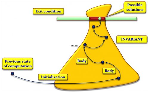
We identify an often large (i.e. very general) area where we know the solution will lie; we call that area the loop invariant. The solution or solutions (there may be more than one) will have to satisfy a certain condition; we call it the exit condition. From wherever we are, we shoot into the invariant region, using an appropriate operation; we call it the initialization. Then we execute as many times as needed (maybe zero if our first shot was lucky) an operation that gets us closer to that goal; we call it the loop body. To guarantee termination, we must have some kind of upper bound of the distance to the goal, decreasing each time discretely; we call it the loop variant.
This explanation is only an illustration, but I hope it makes the ideas intuitive. The key to a loop is its invariant. As the figure suggests, the invariant is always a generalization of the goal. For example, in binary search (and many other search algorithms, such as sequential search), our goal is to find a position where either x appears or, if it does not, we can be sure that it appears nowhere. The invariant says that we have an interval with the same properties (either x appears at a position belonging to that interval or, if it does not, it appears nowhere). It obviously includes the goal as a special case: if the interval has length 1, it defines a single position.
An invariant should be:
- Strong enough that we can devise an exit condition which in the end, combined with the invariant, gives us the goal we seek (a solution).
- Weak enough that we can devise an initialization that ensures it (by shooting into the yellow area) easily.
- Tuned so that we can devise a loop body that, from a state satifying the invariant, gets us to a new one that is closer to the goal.
In the example:
- The exit condition is simply that the interval’s length is 1. (Technically, that we have computed Result as the single interval element.) Then from the invariant and the exit condition, we get the goal we want.
- Initialization is easy, since we can just take the initial interval to be the whole index range of the array, which trivially satisfies the invariant.
- The loop body simply decreases the length of the interval (which can serve as loop variant to ensure termination). How we decrease the length depends on the search strategy; in sequential search, each iteration decreases the length by 1, correct although not fast, and binary search decreases it by about half.
The general scheme always applies. Every loop algorithm is characterized by an invariant. The invariant may be called the DNA of the algorithm.
To demonstrate the relevance of this principle, my colleagues Furia, Velder, and I published a survey paper [6] in ACM Computing Surveys describing the invariants of important algorithms in many areas of computer science, from search algorithms to sorting (all major algorithms), arithmetic (long integer addition, squaring), optimization and dynamic programming (Knapsack, Levenshtein/Edit distance), computational geometry (rotating calipers), Web (Page Rank)… I find it pleasurable and rewarding to go deeper into the basis of loop algorithms and understand their invariants; like a geologist who does not stop at admiring the mountain, but gets to understand how it came to be.
Such techniques are inevitable if we want to get our programs right, the topic of this article. Even putting aside the Bloch average-computation overflow issue, I started with 5 program attempts, all kind of friendly-looking but wrong in different ways. I could have continued fiddling with the details, following my gut feeling to fix the flaws and running more and more tests. Such an approach can be reasonable in some cases (if you have an algorithm covering a well-known and small set of cases), but will not work for non-trivial algorithms.
Newcomers to the concept of loop invariant sometimes panic: “this is all fine, you gave me the invariants in your examples, how do I find my own invariants for my own loops?” I do not have a magic recipe (nor does anyone else), but there is no reason to be scared. Once you have understood the concept and examined enough examples (just a few of those in [6] should be enough), writing the invariant at the same time as you are devising a loop will come as a second nature to you.
As the fumbling attempts in the first few sections should show, there is not much of an alternative. Try this approach. If you are reaching these final lines after reading what preceded them, allow me to thank you for your patience, and to hope that this rather long chain of reflections on verification will have brought you some new insights into the fascinating challenge of writing correct programs.
References
[1] Nadia Polikarpova, Julian Tschannen, and Carlo A. Furia: A Fully Verified Container Library, in Proceedings of 20th International Symposium on Formal Methods (FM 15), 2015. (Best paper award.)
[2] Martin Nordio, Cristiano Calcagno, Peter Müller and Bertrand Meyer: A Sound and Complete Program Logic for Eiffel, in Proceedings of TOOLS 2009 (Technology of Object-Oriented Languages and Systems), Zurich, June-July 2009, eds. M. Oriol and B. Meyer, Springer LNBIP 33, June 2009.
[3] Boogie page at MSR, see here for publications and other information.
[4] Z3 was also originally from MSR and has been open-sourced, one can get access to publications and other information from its Wikipedia page.
[5] Carlo Furia, Bertrand Meyer and Sergey Velder: Loop invariants: Analysis, Classification and Examples, in ACM Computing Surveys, vol. 46, no. 3, February 2014. Available here.
[6] Dynamic programming is a form of recursion removal, turning a recursive algorithm into an iterative one by using techniques known as “memoization” and “bottom-up computation” (Berry). In this transformation, the invariant plays a key role. I will try to write this up some day as it is a truly elegant and illuminating explanation.